Introduction to Stochastic Differential Equations: Why They Matter

The innate randomness within time series data, especially in real-world modeling such as financial time series where we have volatile stock markets, or unpredictable climate patterns, is a major hindrance to accurate predictive modeling. Stochastic differential equations (SDEs) provide a mathematical framework to model such systems by coupling deterministic trends with random fluctuations in data. In their seminal book, Numerical Solution of Stochastic Differential Equations, Peter E. Kloeden and Eckhard Platen offer a comprehensive guide to solving SDEs numerically, making them accessible for applications in finance, physics, and Environmental, Social, and Governance (ESG) modeling. This post introduces SDEs and how to solve them numerically, then we demonstrate its use in modeling stock prices and renewable energy adoption, with simulations done in both F# and Python to bring the concepts to life.

What Are Stochastic Differential Equations?

SDEs are differential equations that incorporate randomness, typically via Brownian motion—a mathematical model of random fluctuations. Unlike deterministic differential equations (e.g., $$( \frac{dx}{dt} = rx )$$ for exponential growth), SDEs account for uncertainty. A general SDE is written as:

$$ dX_t = a(X_t, t) dt + b(X_t, t) dW_t $$

Here, $$( X_t )$$ is the system’s state at time $$( t )$$, $$( a(X_t, t) dt )$$ is the deterministic “drift” (predictable change), and $$( b(X_t, t) dW_t )$$ is the stochastic “diffusion” (random change), driven by Brownian motion $$( W_t )$$. Since analytical solutions are often infeasible, numerical methods like those detailed in Kloeden and Platen’s book are essential for practical simulations.

SDEs are crucial for modeling systems where uncertainty is a key factor. This way we are able to introduce some sense of realism as the models capture random shocks (like market volatility or weather changes), and their numerical solutions enable simulations where the exact solutions are infeasible. They can therefore be broadly applied to different domains like in finance (option pricing), physics (particle motion), and biology (population dynamics). In ESG contexts, SDEs help quantify risks and opportunities, such as sustainable investments or renewable energy growth.

The Euler-Maruyama Method: A Simple Way to Solve SDEs

Solving SDEs numerically is often necessary, and the Euler-Maruyama method is one of the simplest and most widely used approaches. Think of it as an extension of the Euler method for ordinary differential equations, adapted to handle the random term in SDEs.

For an SDE like $$ dX_t = a(X_t, t) dt + b(X_t, t) dW_t $$, the Euler-Maruyama method approximates the solution over small time steps $$ \Delta t $$. Starting from an initial value $$ X_0 $$, it computes the next value $$ X_{t+\Delta t} $$ as:

$$ X_{t+\Delta t} = X_t + a(X_t, t) \Delta t + b(X_t, t) \Delta W_t $$

Here, $$ (\Delta W_t) $$ is a random increment drawn from a normal distribution with mean 0 and variance $$ (\Delta t) $$, simulating Brownian motion. By repeating this over many time steps, we generate a path that approximates the SDE’s solution. The method is straightforward but may require small time steps for accuracy as larger steps can introduce errors (explored in later chapters of the book).

This method is ideal for beginners because it’s intuitive and easy to implement, yet powerful enough for real-world applications like stock price modeling or ESG scenarios. Let’s see it in action with two examples.

SDEs in Action

With a basic understanding of SDEs, let’s check out how we can actually use them to model time series data. We’ll apply the Euler-Maruyama method to the geometric Brownian motion (GBM) SDE:

$$ dS_t = \mu S_t dt + \sigma S_t dW_t $$

This models systems with proportional growth and volatility, perfect for stock prices and ESG applications like renewable energy adoption. We’ll use F# for simulations and FSharp.Plotly for visualizations.

1. Stock Price Simulation (Single Path)

In finance, GBM models stock prices, where $$ (S_t) $$ is the price, $$ (\mu) $$ is the expected return, and $$ (\sigma) $$ is volatility. Below is F# code to simulate a single stock price path using Euler-Maruyama.

open System

// Define Random extension for Gaussian random numbers
type Random with
    member this.NextGaussian() =
        let u1 = this.NextDouble()
        let u2 = this.NextDouble()
        sqrt (-2.0 * log u1) * cos (2.0 * Math.PI * u2)

// Euler-Maruyama for GBM (single path)
let eulerMaruyamaStock (mu: float) (sigma: float) (S0: float) (T: float) (N: int) =
    let dt = T / float N
    let rng = Random()
    let sqrtDt = sqrt dt
    let times = [0.0 .. dt .. T]
    let rec simulate (t: float) (S: float) (path: float list) =
        if t >= T then List.rev path
        else
            let dW = sqrtDt * rng.NextGaussian()
            let S_new = max 0.0 (S + mu * S * dt + sigma * S * dW)
            simulate (t + dt) S_new (S_new :: path)
    (times, simulate 0.0 S0 [S0])

// Simulate stock price: mu = 0.1 (10% return), sigma = 0.2 (20% volatility), S0 = 100, T = 1 year, N = 100 steps
let (times, stockPath) = eulerMaruyamaStock 0.1 0.2 100.0 1.0 100
printfn "Stock price path: %A" stockPath

// Plot the stock price path
let stockChart =
    Chart.Line(times, stockPath, Name="Stock Price Path ($)")
    |> Chart.withXAxisStyle ("Time (Years)")
    |> Chart.withYAxisStyle ("Stock Price ($)")
    |> Chart.withTitle "Simulated Stock Price Path"
Chart.show stockChart

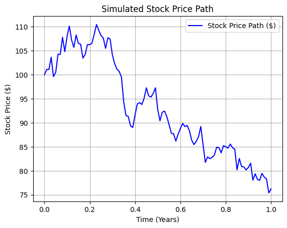
This simulates a stock price starting at Ksh. 100 with a 10% annual return and 20% volatility. The max 0.0 ensures non-negative prices. The results are as:

stock price path: [
   100.0, 101.11301460741727, 101.10552216008797, 103.66038984679442, 99.60423208032427,
   100.52153555846961, 104.28670352879755, 104.2411963925629, 107.81653555108797, 104.82101673954645,
   107.97151860052547, 110.16060759513196, 107.23791032644421, 105.71024891598087, 108.27846467450969,
   106.53674733609895, 106.37217900448393, 103.47916375576835, 104.24743895585692, 106.29036912629937,
   106.26481380560035, 106.59640744591127, 108.48843510122286, 110.47151313733261, 109.21235109360083,
   108.16943390269378, 107.63970939094808, ...
]

The FSharp.Plotly code generates an interactive line plot of the path as shown below:

2. ESG Application: Renewable Energy Adoption (Multiple Paths)

In ESG, GBM can model renewable energy adoption (e.g., installed capacity in gigawatts), where $$ (S_t) $$ is the capacity, $$ (\mu) $$ is the growth rate (policy or technology-driven), and $$ (\sigma) $$ is volatility (market or regulatory uncertainty). Below is Python code to simulate 100 paths and compute statistics.

import numpy as np
import matplotlib.pyplot as plt

# Parameters
mu = 0.05      # Drift (5% growth)
sigma = 0.15   # Volatility (15%)
S0 = 100.0     # Initial capacity (GW)
T = 1.0        # Time horizon (1 year)
N = 100        # Number of time steps
num_paths = 100  # Number of paths
dt = T / N     # Time step size

# Time points (0 to 1 year, 101 points for N=100 steps)
times = np.linspace(0, 1, N + 1)

# Euler-Maruyama for GBM (multiple paths)
def euler_maruyama_esg(mu, sigma, S0, T, N, num_paths):
    dt = T / N
    sqrt_dt = np.sqrt(dt)
    rng = np.random.default_rng()
    paths = []
    
    for _ in range(num_paths):
        path = [S0]
        S = S0
        for _ in range(N):
            dW = sqrt_dt * rng.normal()
            S_new = max(0.0, S + mu * S * dt + sigma * S * dW)
            path.append(S_new)
            S = S_new
        paths.append(path)
    
    return times, paths

# Calculate mean and standard deviation of final values
def stats_final_values(paths):
    final_values = [path[-1] for path in paths]
    mean = np.mean(final_values)
    std_dev = np.std(final_values)
    return mean, std_dev

# Simulate 100 paths
times, paths = euler_maruyama_esg(mu, sigma, S0, T, N, num_paths)

# Calculate statistics
mean_final, std_dev_final = stats_final_values(paths)

# Print results
print("Sample path:", paths[0])
print(f"Mean final capacity: {mean_final:.2f} GW, Std Dev: {std_dev_final:.2f} GW")

# Plot five sample paths
plt.figure(figsize=(10, 6))
colors = ['blue', 'red', 'green', 'orange', 'purple']
for i in range(5):
    plt.plot(times, paths[i], label=f'Path {i+1}', color=colors[i])

plt.title("Simulated Energy Capacity (Gw)")
plt.xlabel("Time (Years)")
plt.ylabel("Capacity (GW)")
plt.grid(True)
plt.legend()
plt.show()

This simulates 100 paths of renewable energy capacity starting at 100 GW, with 5% growth and 15% volatility. The statistics (mean and standard deviation) quantify expected growth and uncertainty.

Sample path: [100.0, np.float64(99.204485180959), np.float64(99.99447815591483), np.float64(98.39472934862667), np.float64(101.73235973308168), np.float64(100.18825614908017), np.float64(100.69041120131182), np.float64(101.1817296020377), np.float64(99.10457879727646), np.float64(100.62659955255305), np.float64(101.63562829880757), np.float64(101.54229485240586), np.float64(100.03065108502152), np.float64(100.11976172211635), np.float64(100.09426848131567), np.float64(101.03939760953821), np.float64(103.8064025910638), np.float64(104.83096431124694),...]
Mean final capacity: 105.69 GW, Std Dev: 15.33 GW

We can visualize five sample paths for clarity:

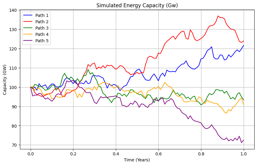
The ESG example models renewable energy adoption, capturing uncertainties like policy changes or market shifts. The mean final capacity (e.g., ~105 GW) and standard deviation (e.g., ~15 GW) inform investment decisions for wind or solar projects, aligning with net-zero goals. Of course we can also use Monte Carlo methods to enhance these predictions by averaging multiple paths.

The stock price example applies to ESG-focused assets like green bonds. Simulating price paths helps assess risks (e.g., Value-at-Risk) for sustainable portfolios, ensuring compliance with governance standards.

Conclusion

Stochastic differential equations are essential for modeling systems with randomness such stock prices or renewable energy adoption. The Euler-Maruyama method makes SDEs accessible, as shown in our F# simulations and plots for stock prices and renewable energy adoption. Run the code with FSharp.Plotly to explore these scenarios interactively. In our next post, we’ll dive into the Itô vs. Stratonovich debate, exploring how these frameworks shape SDE solutions and their applications.

Carlvin Jerry Mwange

Introduction to Stochastic Differential Equations